Table of contents 1. Theoretical background 1.1. Calculating of the antenna input circuit as an example for U4223 1.2. Input circuits 1.3. Ferrite material 1.4. Comparison of the achieved sensitivity with different ferrite antennas 1.5. Receiving direction of root antennas 2. Practical antenna design 3. Summarisation 4. General Hints for troubleshooting 5. Software decoding Hints Back

NEW ! Antenna Calculator NEW !

	Theoretical background

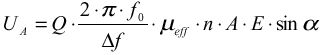
In most cases the design of a radio controlled clock receiver will determine the dimensions of the required receiving aerial for the low frequency band, because the prescribed dimensions must not be exceeded. Usually the aerials work according to the principle of a magnetic dipole, their size can be reduced largely by insertion of a ferromagnetic material. Compared to the antennas for reception of the electrical field the magnetical aerials have the advantage that - regarding the frequency range of interest - they can be easily matched to the input circuit of the receiver. By completion with a parallel-connected capacitor a parallel resonant circuit is originated, which can be tuned to resonance and which allows to adjust noise or impedance matching. Herewith the voltage of the antenna input circuit, which is induced in the antenna coil by the electromagnetic field of the transmitter, is increased with the quality factor Q. It is presumed, that the input impedance of the receiver is high - like that of the integrated circuits T4223B and CME6005 manufactured by ATMEL Germany.

The terminal voltage of the ferrite aerial is determined by several parameters. It can be calculated with the following formula:

(1)

with:
UA = terminal voltage
Q = circuit quality factor
Df = 3 dB bandwidth
µeff = effective permeability
n = number of turns
A = cross-sectional area of the conductor loops
E = electrical field strength at the receiving position
α = angle of the magnetic field referred to the axis of the aerial

The discussion of formula (1) shows, that:

• the electromagnetic field of the transmitter at the receiving position is important
• a directional effect exists
• the induced voltage is higher with thicker ferrite rods
• the ferromagnetic material has an influence
• high numbers of turns lead to high antenna voltages
• a high quality factor increases the antenna voltage

Additionally it should be mentioned that the selectivity of the antenna circuit increases with a raising quality factor Q, which improves the noise immunity regarding reception on adjacent frequencies due to reducing the bandwidth.

For the practical dimensioning of the antenna input circuit it is bear in mind that the different parameters partly are depending on each other. On the one hand a higher number of turns or a increased cross-sectional area effects a higher inductance, on the other hand - provided that the diameter of the wire is the same - it leads to a larger ohmic resistance. With a raising number of turns the antenna voltage grows, but the also increased ohmic resistance counteracts against the raising of the quality factor (see formula 5). Further the effective permeability depends of the realisation of the winding, as the placement on the ferrite rod and the distance from the core. That means that the realisation of the aerial must be optimised for every application (see also section "practical antenna design "). Concerning the directivity, this is an unwanted effect especially for applications, which can't be turned or moved.

For those applications special antenna designs have to be used, which provide an elliptical or omni directional receiving characteristic. The latter can only be achieved with rod aerials. More detailed explanations can be found in the relevant patent literature e.g. DE 3504 660 C2, DE 37 01 378 C2.

Generally it is to state, that - to consider the worst case - noise matching should be the target, due to the low field strength's that must be expected. Thus the most essential criteria for the electrical dimensioning of the antenna is fixed. The optimal generator resistance of the input circuit, for a tuned antenna this is their resonant resistance, is approximately 180kΩ to 300kΩ for the high resistance receiver T4223 / U4223 and about 50 kΩ to 100 kΩ for the CME6005. The optimal value is not easy to determine, as the matching curve shape is rather flat. This means that a rather large range for the nearly optimal resonant resistance can be permitted.

In the frequency range of interest the required resonant resistance can be realised by adequate dimensioning of the antenna circuit. For two reasons it has turned out to be suitable to set the dimensioning to the low-resistive range of the noise-matching curve. Firstly the required quality factors are easier to achieve and secondly the feedback is reduced.

	1.1. Calculating of the antenna input circuit as an example for U4223

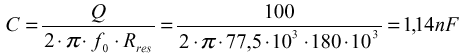
The input impedance of the integrated circuit is neglected. It is high compared to the required generator resistance for optimal noise matching. To reduce feedback the resonant resistance of the antenna circuit shall be set to Rres = 180 kΩ for the U4223.

A quality factor of 100 is realistic and can be achieved without special efforts. The circuit capacitance can be calculated for f= 77,5 kHz (German DCF) as follows (example for the 180 kΩ Antenna):

(2)

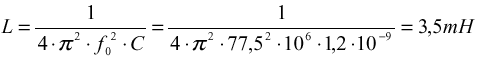
The standard value close to it is: C = 1,2 nF
The corresponding circuit inductance can be found with:

(3)

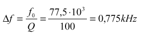
The bandwidth is calculated with:

(4)

If the loss resistance of the capacitor is neglected, the following formula is valid:

(5)

Due to the very small bandwidth of the input circuit exact temperature compensation is essential. For the same reason the aerial must be tuned to resonance with the received time signal transmitter at the actual mounting position. Please note that e.g. metallic objects close to the antenna will influence the alignment and may lead to the necessity of corrections.

Formula (2) can also be used to calculate the resonant resistance Rres if the capacitance is known and the bandwidth Δf is measured. To avoid any influence of components used for coupling between signal generator and antenna, the signal generator should be equipped with a loop antenna for this measurement. The probe that is used to measure the antenna voltage should be an active one. Its resistance must be high compared to the resonant resistance of the antenna and its capacitance must be very small compared to the capacitance of the antenna circuit, so that neither the quality factor nor the resonance frequency of the antenna are influenced in a significant way.

This calculation can also be done for the CME6005 with the 40 to 100 kΩ Antenna resonant resistance.

	1.2. Input circuits

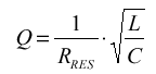
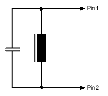
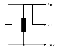
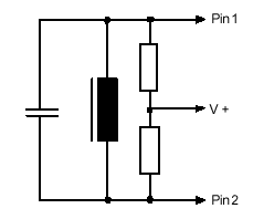
The input stage of the integrated receiver circuit is designed as a differential amplifier. The input transistors must be biased externally in case of the U4223, the CME6005 has in build biasing resistors of 200 kΩ. In the case of U4223 three different input circuits are possible, as figured out in the following circuit diagrams. Please note: the CME6005 can only use a single ended antenna, because of it's in-build biasing resistors (Fig. 1 d).
A balanced connection of the aerial offers the following benefits for the U4223:

• high in-phase suppression
• lower sensitivity against static irradiation
• lower unwanted feedback and therefore less critical construction

A single-ended antenna requires less expenditure.

Different connections of the aerial

a) single ended	b) balanced by means of a cetnre-tapped coil
c) balanced by means of two resistors (2,2MΩ proposed	d) single ended antenna

For the U4223 the variation c) is proposed because of the benefits of a balanced connection, while the expenditure for a tapped coil is avoided. The two resistors used to bias the input transistors should be high resistive to conserve the quality factor of the antenna.

	1.3. Ferrite material

Also the ferrite material has an influence to the quality of the antenna. The user is hold to select a material with excellent behaviour in the frequency range from 20 to 120 kHz in order to reduce losses from the ferrite material. (See also section practical antenna design)

	1.4. Comparison of the achieved sensitivity with different ferrite antennas

For the following comparison different aerials were connected to a demo board of the U4223. An RF generator was modulated with the time signals according to the coding of the German DCF77 transmitter. The generator output was fed to a loop antenna, while the investigated receiving antennas were placed in the axis of the loop antenna at a defined distance. The receiver boards were connected with a data processing unit to decode the time information. The sensitivity was defined by the correct decoding of at least two data telegrams out of four. All measurements were carried out in a shielded room (faraday cage) to avoid failures caused by external disturbing sources. Nevertheless the reproducibility of these measurements is critical. Field distortions inside the shielded room may have an influence; therefore the following results should be regarded only as a rough guideline for own antenna developments. The sensitivities are referred to antenna No. 1. The antennas designed for the use with U4223.

It can be clearly seen, that the antenna can increase the system sensitivity significantly if the antenna is designed in the right way. More increase of the sensitivity of the system can be achieved by using different diameters of wire or by using multiwire wires.

	1.5. Receiving direction of root antennas

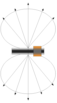
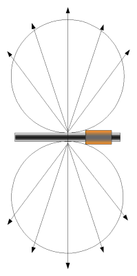
The antennas useful for time code reception, are ferrite-root antennas. This antennas have always a bi-directional receiving behaviour like a classical dipole antenna. (see Figure) By changing the diameter and the length of the root, the characteristic of the reception behaviour can be influenced somewhat. A bigger diameter and a shorter length leads to a less strong bi-directional reception. This information should be taken into consideration by planing the antenna together with the part in which the antenna should work.

Root with short length and bigger diameter	Root with long length and thin diameter

	2. Practical antenna design

Step 1

The CME6005 is designed to be used with a simply antenna, following the Figure 1d).
The resonant resistance Rres should be in the range of 40 to 100 kΩ. Out of the formula (5) we can calculate
the resonant resistance Rres

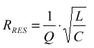
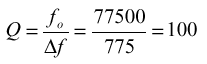
Essential for the Rres is the quality factor Q and the L/C ratio.
To avoid a lot of complicated calculations, we have to use some measurements.
The quality factor Q can be found by measuring the voltage oft the resonant frequency from the antenna and the both corner frequencies with 3 dB (0,707 times) less voltages. This both corner-frequencies give us the bandwidth (3 dB bandwidth = Δf ).

For example: we have the resonant frequency of DCF77 = 77500Hz and a bandwidth of 775 Hz, then we use the simple formula coming from (4):

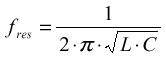
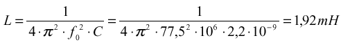
In this case the Q-factor is 100

Step 2

To find the values for the inductance and the capacitance we have to use the formula for a resonant circuit:

Also here we chose a practical value for the capacitance.
The value are mainly between 2,2 nF and 10 nF. The loss factor of the capacitance has to be low (0,0005 tanδ) Out of this assumption we can calculate the value of the inductivity out of (3):

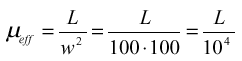
Step 3

Now we need to choose the ferrite material in order to calculate our windings.
The ferrite should have a permeability (µ) of 2000 (real values can differ, also 1800 is ok) and has to be good for frequencies from about 20 to 120kHz to avoid losses in the ferrite material itself. We have also to take in account the temperature factor of the ferrite. This is not a big issue with low quality factors (~50) but with quality factors of 100 and up we have to care, that with changing temperature the resonant frequency of our tuned antenna will not move, because the bandwidth of a antenna with high quality factor (means a good antenna) is small compared with low Q-factors.

Step 4

We need now to know the effective permeability (µeff) of the ferrite material. If we cannot get it from the data's from the supplier, we can get the value easy by putting 100 windings onto the ferrite and than testing the inductance. The following formula shows the way how to get this factor:

The inductance is calculated by:

L= Inductance µeff = effective permeability w = number of windings

If we calculate with 100 windings

To calculate the necessary windings we use:

Step 5

The wire material and the type of doing the windings have an influence to the quality of the antenna.
If we have no limitation of the area where we can bring up the windings, the diameter should be 0,28 mm.
If we have a limitation of the area for windings the whole possible area has to be used in order to decrease the wire diameter not below 0,15 mm. From formula (5) can be seen that a reducing of the antenna capacitor leads to a higher necessary inductance this will increase the effective antenna voltage and also the resonant resistance. The higher necessary windings on the ferrite lead to more losses due to spread capacities between the windings and therefore a decreasing of the quality factor Q. If there is a necessity to use a high number of turns, the reducing of the thickness of the isolation of the wire can be taken in account. The same number of windings and the same diameter of the wire can lead to different Q factors if the isolation and the accuracy of the windings are changed.

Step 6

In all cases, the antenna has to be tuned to the desired frequency, because the ferrite itself as well as the capacitor have some tolerances. The easiest way is to make the coil movable on the ferrite. The capacitor has it's best place on the windings or as close as possible to the coil. A phase-gain analyser is the ideal tool to very quickly find the resonant point. Now moving the coil on the ferrite varies the resonant frequency to the desired value e.g. 77500kHz (DCF77).
This test can also be done according the description in the datasheet. In this case the capacitance of the test-probe has to be taken in account. This capacitance detunes the antenna.
A more difficult way is to measure the antenna in conjunction with an application board of the CME6005. The voltage at the capacitor PK is a value of the input-voltage from the antenna. By measuring the voltage at this point, the antenna can be optimised. Essential is that this is done in a faraday cage to avoid any influence from other carriers. This test point (PK) shows the sum of all frequencies the antenna catches. It is easy to understand that each distortion leads to a wrong result. A variation of the L/C of the antenna can lead also to more optimized results.

	3. Summarisation

If all the above mentioned points are taken into account, it is still good, to do some variations of the antenna in order to find the antenna with the best result in the specific application.
For the most important frequencies the following dimensioning results in usable antennas, but not optimised to a specific application.

The quality factor this dimensioning was based on can be achieved only with high-quality capacitors.
To avoid feedback, the connecting wires to the aerial should be shielded or at least twisted.

	4. General hints for troubleshooting

The antenna is mainly sensitive to the magnetic component of the transmitted frequency. There are a lot of possible external and internal electrical and magnetically distortions. Thus, close to the antenna any wire with AC components on it has to be avoided. This is also valid for the output of the receiver. The receiver is a direct receiver and components from the output signal, coupled to the antenna by electrical field or parasitic capacitors, cause a reduction of the sensitivity. The leads of the antenna has to be shielded or at least twisted to avoid unsymmetrical induction of noise. Also metal component e.g. batteries, holder for batteries, detune the antenna and reduce the sensitivity of the system. LCD display have a extensive field of distortion. This components have to be placed as fare as possible from the antenna AND receiver.
Special attention has to be given to micro-controller. They produce a high noise level with high slope rates. These high slope rates can interfere to the antenna and lead to a short ringing of the antenna, this results in a sensitivity decrease of the system.
The low pass filter of the Vcc for the micro-controller is also a point which creates noise.

Summarisation:

• Place antenna far away from electronic components which create interference e.g. processor, display, signal lines....
• Place antenna minimum 20 mm away from metallic parts e.g. batteries
• If you measure at U4223, pin REC, INT or DEC you must use a test probe with impedance higher than 1 GΩ. This is also good for testing CME6005 pin PK
• Use separate power supply lines for receiver, processor and display.
• Use RC combination to block any distortion on Vcc.
• Use only one central ground point for the receiver.
• Make short connection from the crystals to the receiver (avoid additional wire capacity)
• Avoid any current loops as well as ground loops nearby the IC.
• Provide shielding under the IC with ground layer of PCB if possible.

	5.Software decoding Hints

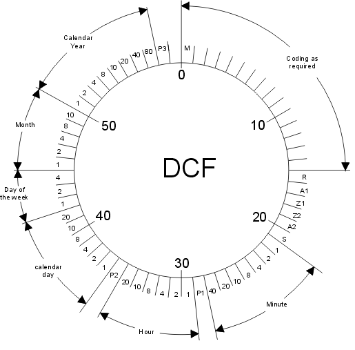
The time code signal generally has the following format:

Each second is 1 bit transmitted. The place of the bit (1 to 59) gives the meaning of the information of this bit.

Example:

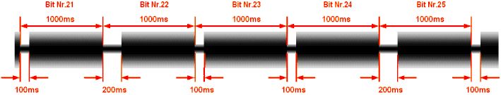
The signal at the antenna looks like that:

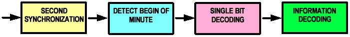
To decode a Time-Code-Signal several principal steps are necessary.

To do the information-decoding, the coding of the transmitter used has to be taken. Examples can be taken out of the datasheet.

Please note: The user is responsible to verify the information from the transmitters. If the coding changes, no warning is given from the submitter of the paper.